Optuneでパラメータ最適化、ランダムフォレスト、XGB、LGBM分類器でアンサンブル

ライブラリ、データ読み込み
内容確認
前処理
データ探索
モデル作成
参考

ライブラリ、データ読み込み

まずは、必要なライブラリや、データの読み込みを行いましょう。

import numpy as np 
import pandas as pd 
import sklearn
import random
import warnings

pd.plotting.register_matplotlib_converters()
import matplotlib.pyplot as plt
%matplotlib inline
import seaborn as sns

train_data = pd.read_csv("/kaggle/input/icr-identify-age-related-conditions/train.csv",index_col="Id")
test_data = pd.read_csv("/kaggle/input/icr-identify-age-related-conditions/test.csv",index_col="Id")
train_data.head()

内容確認

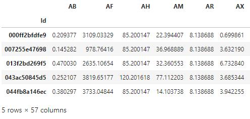
データセットの内容は、すべて匿名化されております。

前処理

データEJだけは、object型なので数値化し、そのほかのデータに関しても、NaNがあれば取り除きます。

meanTrain = train_data.mean()
meanTest = test_data.mean()

for i in train_data.columns:
    if i!="EJ":
        train_data[i].replace(to_replace=np.NaN,value=meanTrain[i],inplace=True)
        
for i in test_data.columns:
    if i!="EJ":
        test_data[i].replace(to_replace=np.NaN,value=meanTest[i],inplace=True)
    else:
        test_data[i].replace(to_replace=np.NaN,value=1,inplace=True)
        
max(train_data.isnull().sum())

from sklearn.preprocessing import LabelEncoder

encoder = LabelEncoder()

train_data["EJ"] = encoder.fit_transform(train_data["EJ"])
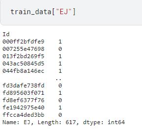
test_data["EJ"] = encoder.transform(test_data["EJ"])

データEJに対して、質的変数から数値データに変換するために、LabelEncoder()を使います。このメソッドでほかの変数と同様に数値データとして扱うことが出来ます。

データ探索

ここでは、データセットの内容をより深く見てみます。

colsFloat = train_data.select_dtypes("float64").columns
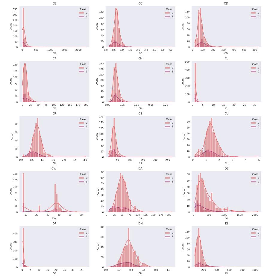
colsInt = train_data.select_dtypes("int64").columns

試しにデータABに対するクラス0とクラス1の分布を見ます。

fig, axes = plt.subplots(1,1,figsize=(10, 10))
data = "AB"
sns.histplot(train_data,x=data,hue="Class",bins=40,kde=True,palette="flare");
plt.gca().set_title(data)
    
fig.tight_layout()
plt.show()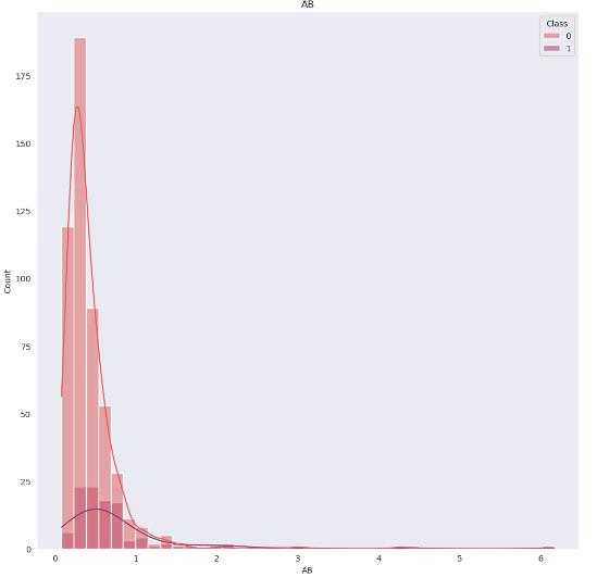

同じような傾向を示しており、ABの値を見るだけでは分類は出来なそうです。

一つずつ見るのも大変なので、まとめて表示して傾向を調べてみます。

fig, axes = plt.subplots(19,3,figsize=(15, 60))

for i in range(len(colsFloat)):
    plt.subplot(19,3,i+1)
    sns.histplot(train_data,x=colsFloat[i],hue="Class",bins=40,kde=True,palette="flare");
    plt.gca().set_title(colsFloat[i])
    
for j in range(len(colsInt)):
    plt.subplot(19,3,i+j+2)
    sns.countplot(train_data,x=colsInt[j],palette="flare");
    plt.gca().set_title(colsInt[j])
    
fig.tight_layout()
plt.show()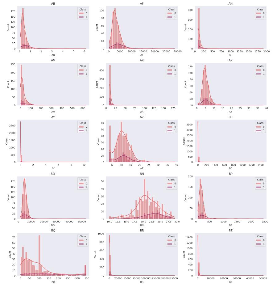

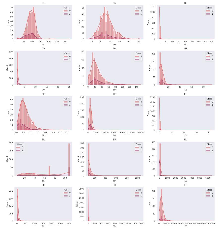
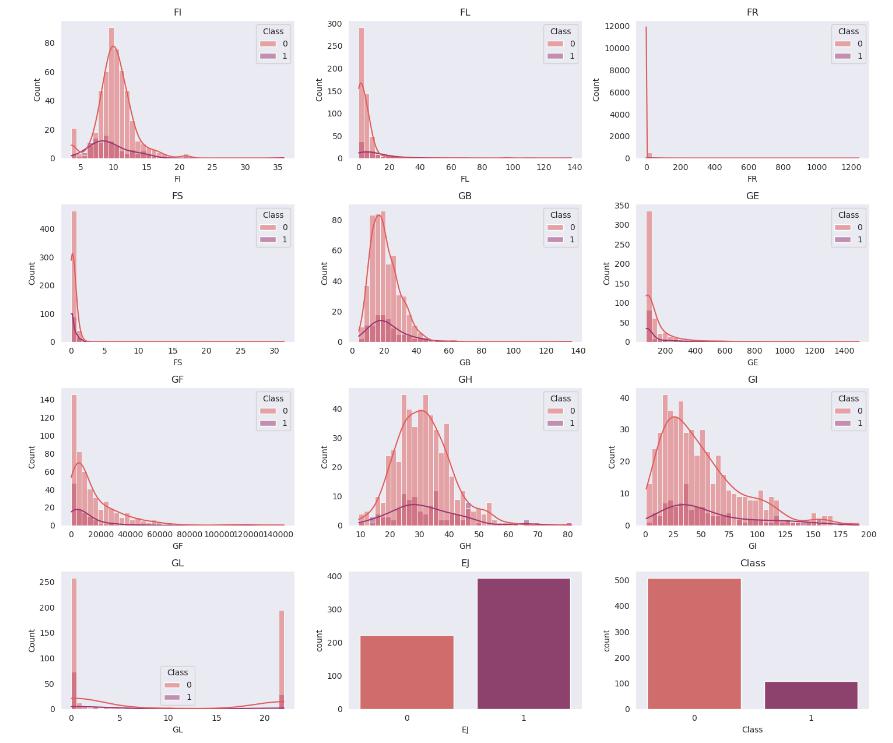
どのデータを見ても、二値分類を行うのは難しそうです。
次は、各データ間の相関をヒートマップで示してみます。

features = [i for i in train_data.columns]
corr = train_data[features].corr(numeric_only=False)
plt.figure(figsize = (20,20))
sns.heatmap(corr, cmap = 'rocket', annot = False,vmin=0);
plt.show()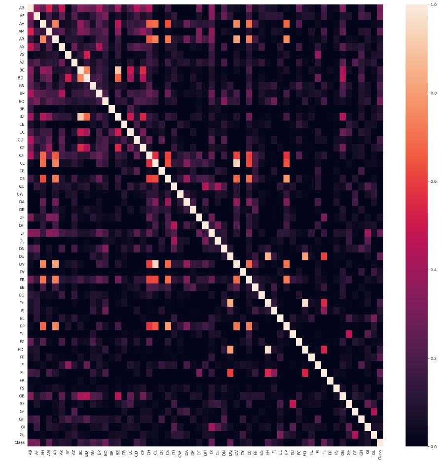

モデル作成

ここでは、モデルを作成するために必要なモジュールのインポートを行います。

from catboost import CatBoostClassifier, Pool
from xgboost import XGBClassifier
from lightgbm import LGBMClassifier
from sklearn.model_selection import train_test_split, cross_val_score, GridSearchCV, cross_validate
from sklearn.metrics import accuracy_score, roc_auc_score, confusion_matrix
from sklearn.ensemble import RandomForestClassifier
from sklearn.ensemble import GradientBoostingClassifier
from sklearn.ensemble import VotingClassifier
from sklearn.ensemble import HistGradientBoostingClassifier
import optuna

データセットを訓練用とテスト用に分けます。
入力にはClass以外のデータを使い、出力はClassのデータを使います。20%のデータをテストデータとし、残りの80%を訓練データとして用います。

cols = [i for i in train_data.columns if i!="Class"]
seed = np.random.seed(6)

X = train_data[cols]
y = train_data["Class"]

X_train, X_test, y_train, y_test = train_test_split(X,y, test_size=0.20,random_state=seed)

まずは、ランダムフォレストでの分類を行います。

 def objective(trial):
     params = {
         "max_depth":trial.suggest_int('max_depth',3,10),
         'n_estimators' : trial.suggest_int('n_estimators',100,2500),
         "min_samples_split": trial.suggest_int('min_samples_split', 2,8),
         "min_samples_leaf" : trial.suggest_int('min_samples_leaf', 1,5),
         "max_features": trial.suggest_categorical("max_features",["sqrt", "log2", None]),}
     rfmodel_optuna = RandomForestClassifier(**params,random_state=seed,criterion="log_loss")
     rfmodel_optuna.fit(X,y)
     cv = cross_val_score(rfmodel_optuna, X, y, cv = 4,scoring='neg_log_loss').mean()
     return cv

 study = optuna.create_study(direction='maximize')
 study.optimize(objective, n_trials=100,timeout=2400)

ハイパーパラメータとして、決定木の層の深さや木の数を決める必要があります。今回は、ハイパーパラメータを決めるために、Optunaを利用します。

[I 2023-07-09 15:30:21,506] Trial 31 finished with value: -0.2180754236196637 and parameters: {'max_depth': 8, 'n_estimators': 2401, 'min_samples_split': 4, 'min_samples_leaf': 2, 'max_features': None}. Best is trial 24 with value: -0.2175296838433788.

上記のような結果を得られるので、このハイパーパラメータを投入して、モデルの学習を行います。ハイパーパラメータ自体はベイズ統計を活用して求められているので、試行回数を同じにしても、常に同じ値を返すとは限りません。

params = {'max_depth': 8, 'n_estimators': 2401, 'min_samples_split': 4, 'min_samples_leaf': 2, 'max_features': None}

rfmodel = RandomForestClassifier(**params,random_state=seed,criterion="log_loss")
rfmodel.fit(X_train,y_train)

訓練済みのモデルはrfmodelに入っているので、一旦、そのままにし、ほかのモデルでの学習を行います。

次に、XGB分類器でのモデルの学習を行います。
先ほどと同様に、Optuneを利用してハイパーパラメータの最適化を行っていきます。

def objective(trial):
    params = {
    'n_estimators' : trial.suggest_int('n_estimators',2000,3000),
    'max_depth':  trial.suggest_int('max_depth',3,8),
    'min_child_weight': trial.suggest_float('min_child_weight', 2,4),
    "learning_rate" : trial.suggest_float('learning_rate',1e-4, 0.2),
    'subsample': trial.suggest_float('subsample', 0.2, 1),
    'gamma': trial.suggest_float("gamma", 1e-4, 1.0),
    "colsample_bytree" : trial.suggest_float('colsample_bytree',0.2,1),
    "colsample_bylevel" : trial.suggest_float('colsample_bylevel',0.2,1),
    "colsample_bynode" : trial.suggest_float('colsample_bynode',0.2,1)}
    xgbmodel_optuna = XGBClassifier(**params,random_state=seed,tree_method = "gpu_hist",eval_metric="logloss")
    xgbmodel_optuna.fit(X,y)
    cv = cross_val_score(xgbmodel_optuna, X, y, cv = 4,scoring='neg_log_loss').mean()
    return cv

study = optuna.create_study(direction='maximize')
study.optimize(objective, n_trials=100,timeout=1200)

LGBM分類器での学習を行います。

def objective(trial):
    params = {
        "num_leaves": trial.suggest_int('n_estimators',20,100),
        "max_depth":trial.suggest_int('max_depth',3,10),
        "learning_rate" : trial.suggest_float('learning_rate',1e-4, 0.2),
        'n_estimators' : trial.suggest_int('n_estimators',100,2500),
        "min_child_weight" : trial.suggest_float('min_child_weight', 0.5,4),
        "min_child_samples" : trial.suggest_int('min_child_samples',10,50),
        "subsample" : trial.suggest_float('subsample', 0.2, 1),
        "subsample_freq" : trial.suggest_int('subsample_freq',0,5),
        "colsample_bytree" : trial.suggest_float('colsample_bytree',0.2,1)}
    lgbmmodel_optuna = LGBMClassifier(**params,random_state=seed,device="gpu")
    lgbmmodel_optuna.fit(X,y)
    cv = cross_val_score(lgbmmodel_optuna, X, y, cv = 4,scoring='neg_log_loss').mean()
    return cv

study = optuna.create_study(direction='maximize')
study.optimize(objective, n_trials=100,timeout=1200)

参考

https://www.kaggle.com/code/iqmansingh/icr-optuna-xgb-lgbm-rf-ensemble-eda

最近の投稿

最近のコメント

アーカイブ

カテゴリー